
Technology: Python, TensorFlow, pandas, numpy Tags: Machine Learning, Data Engineering, Deep Learning, Recommendation Systems Image Credits: Natalie Perea on Unsplash
Track2Seq - LSTM Recommender
Automated playlist continuation has been coined as one of the grand challenges in music recommendation. For my Computer Science master's thesis I decided to tackle this problem by leveraging an approach from natural language processing. The idea is to create a language model based on song or track URIs. The resulting recommendation system is called Track2Seq. Initial experiments on a large scale dataset show an over 24% improvement in r-precision when compared against state-of-the-art recommendation baselines.
Track2Seq is a deep long short-term memory network designed to continue sequences such as music playlists. Code and thesis can be found online.
The Issue
Leading recommendation systems such as collaborative-filtering (CF) can have difficulties dealing with a large amount of data. In addition, CF methods usually have no way of recommending tracks when no seed tracks are available. Track2Seq proposes a way to approximate seed-tracks based on a playlist title only and a recommendation system that can handle sequential information of arbitrary length.
The task at hand was to develop a system that can take in a playlist \(p\) of tracks where the length of each playlist \(|p| \in \{0, 1, 5, 10, 25, 100\}\). The summary focuses on the process of training a deep LSTM network and using it to predict a playlist continuation.
Dataset
The data was taken from Spotify's million playlist dataset (MPD). MPD contains track information of a million playlists. This includes meta-data, title information as well as track and artist names. The initial version of Track2Seq uses only the track uri. Due to computational constraints only tracks that appear more than 5 times were included in the training process. To develop and test the model, the data was split in a development and test set each containing 1% of the playlists (10,000 each). By counting and aggregating track information per playlist it was possible to create a dataset that represents core features of the data at hand. To make sure the distributions mirror the same ground-truth, development and test sets are stratified on three features that are important to the consistency. The process of stratification was done to reflect attributes such as popularity, time and playlist richness which are important features for recommendation systems.
Track2Seq
Track2Seq leverages a training method introduced by Alex Graves. To do so, the data is turned into machine-readable information. Besides meta-data, all playlists of MPD contain a list of tracks. Every track \(t_{i} \in p\) is identified by an URI such as spotify:track:4v6jydWBTAIqnyPVNyOAdc. Those URI can be seen as classes. This allows for the entire vocabulary of tracks to be one-hot-encoded.
The network uses two layers of LSTM cells in a recurrent neural network (RNN) to operate. While this book gives a good mathematical introduction into the world of deep learning, this book offers a nice practical introduction into machine learning and some of the novel concepts. Brief introductions into RNN and LSTM can be found online.
In a nutshell, RNN are a class of networks that can handle sequential information. They do so by introducing backward pointing connections and parameter sharing across time-steps. These features enable RNN to scale to longer sequences than practical for standard feedforward networks. To offer a visual on how a single recurrent perceptron (read artificial neuron) could be portrayed (and to show off my "impeccable" graphing skills) I posted a little graph below. The step function of the unit determines whether it is activated or not. \(w_x\) and \(w_y\) are two parameter weights which are shared across time-steps.
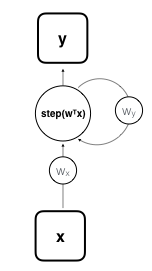
Fig: Recurrent perceptron with one neuron in compact form.
Basic RNN come with some drawbacks. One problem that has been investigated when using RNN is their inability to handle long-term dependencies in sequences. Another issue that is linked to their struggle with long sequences are vanishing or exploding gradients. Vanishing and exploding gradients originate in the recurrent structure. Because weights are shared across all time-steps, the recurrent nature of the network leads to weights and gradients being multiplied with itself. These issues can be alleviated by using specific memory cell structures called LSTM cells.
RNN and LSTM networks work well with sequential information such as time-series information, audio, video, sentences or like in our case music playlists. To get a gist on the concepts needed to understand the Track2Seq implementation, you are always welcome to check out chapter 3 and 4 of my thesis.
Training
One way of training RNN is predicting the next item of a sequence. If those predictions follow a probabilistic distribution it is possible to create novel sequences. By instantiating the trained model with a seed sequence and taking each prediction at a time-step as a potential candidate a stream of recommendations can be initiated. The characteristics of those sequences don't follow an exact template but use interpolations of the internal representation of the tracks. This makes them unique to a degree where generating the same sequence twice is highly unlikely.
To train the model, an encoded seed sequence \(x = (x_1, x_2, x_3, ..., x_t)\) with a target sequence \(y = (x_2, x_3, x_4, ..., x_{t+1})\) that is shifted by one time-step is fed into the neural network
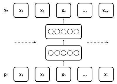
Fig: Training process of network. \(p_n\) consists out of one-hot encoded track sequence. \(y_n\) represents \(p_n\) shifted by \(1\).
To boil it down, the idea is to take all playlists, feed the network sequences from the playlists such as:
\(x =\) Rick Astley - Never Gonna Give You Up, Kim Wilde - Kids In America, Bananarama - Venus, Dead Or Alive - You Spin Me Round
\(y =\) Kim Wilde - Kids In America, Bananarama - Venus, Dead Or Alive - You Spin Me Round, Bronski Beat - Smalltown Boy
Where the last track of \(y\) is the next track in the playlist that appears after sequence \(x\). To say it with the words of any music industry professional: All killer, no filler.
Through this training process, the LSTM network learns a compressed representation (often called embedding) for each track. These embeddings describe the tracks in a vector space with 128 latent features.
Prediction
The prediction process consists out of three main stages: Initialization, prediction and aggregation. The first stage is the initialization stage. Since the prediction network is a RNN with LSTM cells, the network needs to be initialized before predicting. This helps to establish the context of the seed sequence. At the beginning both states are randomly initialized. To continue the initialization process the model feeds the seed sequence in the network once. While doing so, it instantly adds track probabilities to a dictionary of candidates. In addition the first iteration initializes the starting states for the prediction process that follows afterwards.
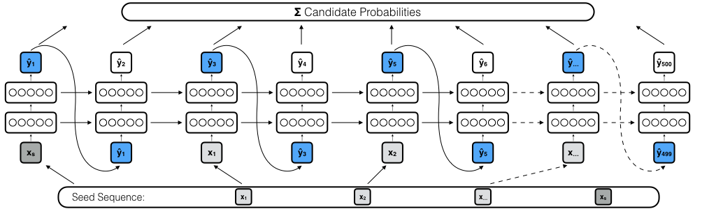
Fig: Semi-guided prediction process of sequence continuation with deep LSTM network. \(\hat{y}_t\) contains top-k most likely candidates at step \(t\) and their probabilities. All probabilities are summed up per candidate over the course of 500 steps. The highest scoring candidates determine the continuation sequence.
After initialization, the prediction stage starts by running the prediction process for \(n\) times. In this stage either a fully- or semi-guided configuration can be chosen to generate a candidate dictionary. The prediction and aggregation stages work in concert. At each prediction step \(k\) tracks with the highest next-item probabilities are collected in a dictionary \(C\). To aggregate a final candidate list, every track \(C_i \notin S\) is added to a dictionary while adding up their probability scores per track. After \(n\) prediction steps, 500 candidates with the highest aggregated probability are returned as recommendations.
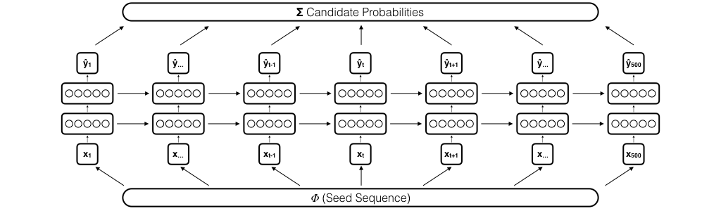
Fig: Fully-guided prediction process of sequence continuation with deep LSTM network. The network receives a randomly drawn seed-item at every time-step. Initialization and aggregation stages are the same as in a semi-guided prediction process.
Results
To validate the results of Track2Seq the best-performing model is compared against two state-of-the-art recommendation baselines. As collaborative filtering baseline weighted matrix factorization (WMF) is used. WMF works well for implicit feedback. The second baseline applies the idea of word2vec (W2V) to perform the recommendation task.
All recommendation systems are evaluated on accuracy (r-precision), relevance (recall), ranking quality (normalized discounted cumulative gain) and a combination of the three (recommended song clicks). A concise definition of the metrics can be found here. To have a ground-truth to test against all development and test playlists are sorted by length and divided into 6 categories of different seed-track lengths \(\{0, 1, 5, 10, 25, 100\}\). All tracks after the seed-track length are hidden and stored as ground-truth.
As mentioned in the opening, the recommendation system is able to approximate seed tracks. This is done through a process called cosine-weighted vector averaging (CWVA). The experiment suggests that for little or no seed-track information this process could outperform all other methods.
| Method | R-Precision | RSC | NDCG | Recall@500 |
|---|---|---|---|---|
| W2V | .0425 | 13.9564 | .1075 | .1696 |
| WMF | .0917 | 7.1087\(^\Delta\) | .2328 | .3775 |
| Track2Seq | .1049\(^\Delta\) | 7.3092 | .2584\(^\Delta\) | .4013\(^\Delta\) |
| Track2Seq & CWVA | .1142 | 5.8766 | .2750 | .4239 |
Tab: Average results for baseline methods and Track2Seq. Best score is marked in bold, \(^\Delta\) indicates the second best score.
- After training Track2Seq for one epoch, the proposed approach achieves the highest average r-precision score. Track2Seq & CWVA improves the best baseline result by over 24%.
- T2S & CWVA has a NDCG of .2750 which is over 19% higher higher than the score for WMF.
- The proposed model has also the highest recall score. T2S & CWVA has a 25% higher score compared to WMF.
- For RSC, where lower scores are better, the proposed model with CWVA achieves a score of 4.69 which is over 35% improvement to the best baseline.
- Even though W2V had competitive scores on the development set, its results for the testing set decreased significantly. The only competitive score was achieved for r-precision and 0-seed playlists.
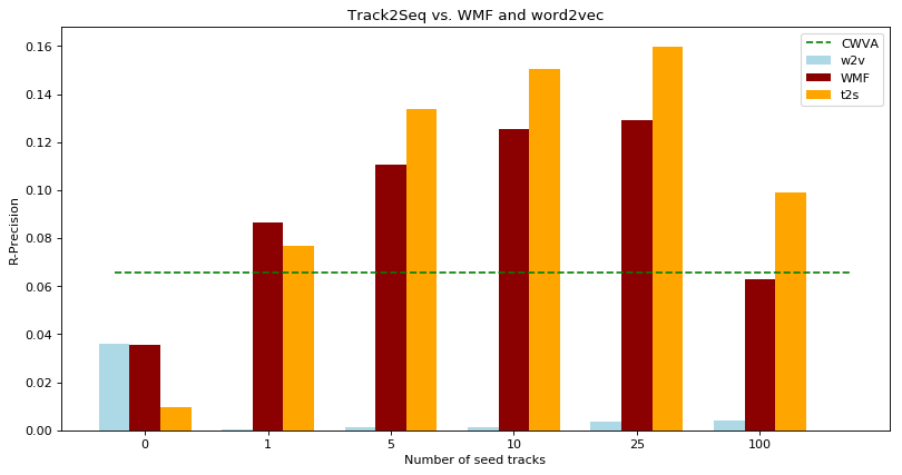
Fig: R-Precision scores per seed-track length. T2S outperforms WMF baseline for all seed lengths but 0-seed and 1-seed playlists. Dashed line indicates the r-precision average for CWVA.
To understand the advantages of all models, their scoring on different sequence lengths is investigated. Surprisingly CWVA outperforms both baselines for long sequences and has a clear advantage over all methods when no seed tracks are available. In general CWVA seems to perform well as a recommendation substitute for 0-seed playlists but the noise that is added to the seed list throws off the T2S network. The score values for 0-seed playlists are quite low in general. When looking at 1-seed playlists, T2S performs just slightly better than WMF. After more information is included T2S generates more precise recommendations than WMF. T2S has the best r-precision score for playlists with a sequence length of 25. Low r-precision scores for playlists with more than 100 tracks could originate also from the skewed training data. The bulk of the playlists contain fewer than 100 tracks with a heavy skew towards playlists with less than 50 tracks.
In the thesis the findings as well as additional metrics and results for different sequence lengths are discussed further.
Track2Seq introduces a way of continuing music playlists using a broad variety of seed information that ranges from only a playlist title to seed sequences of 100 tracks. By leveraging probability outputs, combined with a guided prediction configurations the network is able to improve state-of-the-art recommendation systems.